Wiggett [2] describes the Orton film method roughly as: Using slide film, take one photo of a scene with sharp focus, and overexposed. Then, take a second photo of the same scene, out-of-focus, and also overexposed. Sandwich the two slides together to get the final image.
To convert a single digital image using the Orton effect, we need to find the digital equivalents of this description. Sandwiching two slides together is equivalent to multiplying two digital layers together.
Orton_Image = (Sharp_Overexposed_Image) × (Blurry_Overexposed_Image)
For the first part, we need to take the source image, and apply some function to make it "overexposed." We can use the Photoshop Adjust->Exposure function, but there are other options. For now, let's just refer to the lightening function as LightenS().
Sharp_Overexposed_Image = LightenS( Source_Image )
For the second part, we need to make a blurry copy of the source image, and then lighten it as well. To make an image blurry, we will use a GaussianBlur() function. To lighten this blurry image, we'll use another lightening function referred to as LightenB().
Blurry_Overexposed_Image = LightenB( GaussianBlur( Source_Image ) )
The three equations so far define the 2-Layer Orton method. Wiggett [2] uses a copy of the image screened with itself for the LightenB() and LightenS() functions. Grossman [3] skips the LightenB() and LightenS() steps, and prefers to lighten the final image instead. SomeOtherBob [4] uses Gamma correction with Levels for his LightenB() and LightenS() functions.
3-Layer Orton adds a little more complication to the blurry part of the equation. Instead of using a fully blurry image, it uses a blurry image masked over a sharp image. By selectively masking between the blurry and sharp copies, we can adjust the amount of sharpness retained in parts of the final image. Our last equation becomes:
Blurry_Overexposed_Image = LightenB( ( GaussianBlur( Source_Image ) masking (Source_Image) )
The layer and group structure created with the Actions is the Photoshop representation of these equations. Group 1 is the (Sharp_Overexposed_Image) portion, and contains the sharp image modified by some lightening function. Group 2 is the (Blurry_Overexposed_Image) portion, and it contains the sharp copy, first masked by the blurry copy, and then lightened by another function. Group 2 is set to blending mode "Multiply" to complete the transformation.
All of the digital Orton methods (at least so far as I've seen) can be fit into this structure. The differences between the methods are due to the selection of lightening functions.
Lightening Functions
[Quick note: all of the mathematical disucssions that follow refer to pixel values ranging from 0.0 (black) to (1.0) white. The graphs show input range (0-1) from left to right, and output range (0-1) from bottom to top.]
Why do we need to lighten at all? We're basically multiplying an image against itself. Each pixel (p) becomes (new_p = p × p). Graphically, the result is:
 Sharp Image |
Blur Image |
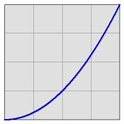 Dark Result |
Think of a 50% grey pixel (p=0.5). The resulting pixel would be (new_p = 0.5 × 0.5 = 0.25) which is 25% grey, much darker than the original. We have to do some sort of lightening, either to the source images or to the resulting image, to counteract this darkening.
Exposure Functions
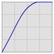
The lightening functions that we choose will have a dramatic effect on the final image. Consider the film technique described by Wiggett [2]. The sharp image is taken at +2.0 exposure, and the blurry image is taken at +1.0 exposure. If we simulate these exposures using the Photoshop Adjust->Exposure tool, we find the images are simply highlight clipped by a certain amount. When the two images are multipled together, the net result is described by the curves here:
 Sharp +2.0 Exposure |
 Blur +1.0 Exposure |
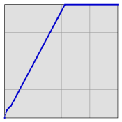
 High Contrast, Blown Highlights |
The result is a very contrasty image, with all pixel values above 75% white completely lost to clipping. This is not necessarily a bad thing, it's just a distinct effect of this method. You can try it on your images using the "Setup - Exposure" action.
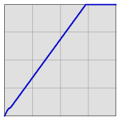
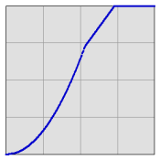
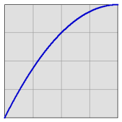
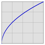
The "Setup - Expcurves" method is based on the exposure effect, with some rounding of the curves to try to save some highlight details. The curves are roughly linear up to output = 75% white. Above that point, the curve is allowed to move smoothly towards 1.0(in) = 1.0(out). The combination that results is still very contrasty, but it doesn't clip the highlight values:
 Sharp + Expcurve 2.0 |
 Blur + Expcurve 1.0 |
 High Contrast, Some Highlights Preserved |
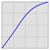
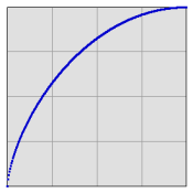
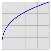
The "Setup - RawExp" method is also based on the film technique. In this case, the lightening curves were produced from RAW image manipulation. The original image was prepared in Camera Raw to a nice even exposure with 100% Recovery of the highlights. The same image was then re-extracted with +1.00 and +2.00 added to the exposure. By comparing these lightened pictures with the neutral exposure, we can determine a curve-approximation to the raw exposure function. When we apply these functions to our method, we get these results:
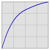 Sharp + Raw Exp 2.0 |
 Blur + Raw Exp 1.0 |
 Slight Contrast, Some Brightening |
The use of 100% Recovery in Camera Raw prevented the image from having blown out highlights, as seen in the lightening curves. The final image is not much more contrasted than the original, but it does get brightened up a bit in the mid-tones and highlights.
Screen Functions
Wiggett [2] suggests lightening your source images by duplicating the image, and then screening the original with the copy. Mathematically, that works out to:
Screen 1/2 function:
new_p = 1 - (1-p)×(1-p) = 2×p - p×p
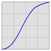
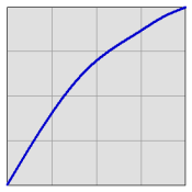
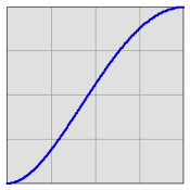
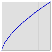
This function is called "Screen 1/2" in the Actions set. The Method that uses this lightening function is "Setup - Screen". When an image is lightened with Screen 1/2 and then multiplied, the resulting image curve looks like this:
 Sharp + Screen 1/2 |
Blur + Screen 1/2 |
 Some Contrast, Highlights Preserved |
The new image is not quite as contrasty as found in the methods above. Hightlight and shadow values are nice and smooth as well, if little compressed.
Note that this pair of functions is symmetric between the sharp and blur sides. (We use the same function on both sides.) Note also that the film method uses more lightening on the sharp image, and less on the blurry image. The difference is subtle in the final image, but you may want to experiment with it. The Action set includes setups for lightening functions called "Screen 1/3" and "Screen 2/3". When these functions are used, the overall shape of the final curve is the same as the "Screen 1/2" pair.
 Sharp + Screen 1/3 |
 Blur + Screen 2/3 |
 Some Contrast, Highlights Preserved |
If you really want to know, the Screen 1/3 and Screen 2/3 functions are derived as:
Screen 1/3 function:
new_p = ((2×p - p×p) × (2×p - p×p)) ^ (1/3)
Screen 2/3 function:
new_p = ((2×p - p×p) × (2×p - p×p)) ^ (2/3)
Gamma Functions
SomeOtherBob [4] suggests using a gamma adjustment for the lightening functions. A gamma function is given by the equation:
new_p = p ^ (1/gamma)
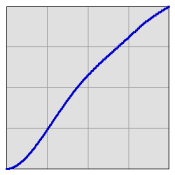
This is an exponential function that conveniently works well with the multiplication that follows. A gamma value of 2.0 is the equivalent of taking the square root of the pixel values. When you multiply two square roots together, you get the original value back again:
 Sharp + Gamma 2.0 |
Blur + Gamma 2.0 |
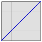 Original Gamma Preserved |
When you want an asymmetric pair of lightening functions, you just have to select the values for gammaS and gamma B according to the equation:
(1/gammaS) + (1/gammaB) = 1
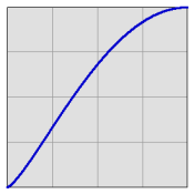
The "Setup - Gamma" method uses a strong gamma of 3.0 for the sharp image, and a weak gamma of 1.5 for the blurry image. Since (1/3.0 + 1/1.5 = 1), this pair works:
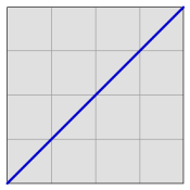
 Sharp + Gamma 3.0 |
 Blur + Gamma 1.5 |
Original Gamma Preserved |
Note that the gamma lightening functions do not do anything to enhance the contrast of the final image. Wiggett suggests that a good Orton Image should have strong, saturated colors. If you use the Gamma method, you may want to add layers to adjust the contrast and saturation of the final result.
Invent Your Own Method
The benefit to the layered setup is that you can change the lightening functions and immediately see the change reflected in the final image. To make your own Orton method, start with one of the methods that uses Curves: Screen or Expcurves. Blur your blur layer to complete the basic effect. Then you can adjust the curve settings in the lightening layers to any effect that you want. If you prefer, remove a curve function with a different adjustment layer: levels for gamma, exposure for that effect, or any other effect you want to try.
All of the discussion above has ignored one thing. The Gaussian Blur function tends to have the effect of reducing the contrast of the blurred image. You might consider adjusting your blur lightening curve to compensate for that compression of pixel range.